Table of contents
Microsoft Excel is a spreadsheet application that offers an extensive suite of features, including tools for data storage, calculation, and Visual Basic programming. Excel is recognized as an industry standard for spreadsheet applications, with millions of diverse users worldwide. As a versatile, feature-rich application, Excel provides a variety of tools and features that are specifically beneficial for academic purposes. The list of tips and tricks below provides solutions to common cell formatting challenges that you may encounter when using Excel.
For more tips and tricks on Excel view the Overview of Basic Tasks and the Excel Ribbon and Working with Formulas in Excel.
Select cells, rows, columns, or worksheets
All data entered into Excel is stored in cells within a worksheet. These cells are arranged into a grid of rows and columns. Excel worksheets can contain 1 million rows and just over 16000 columns. To effectively work with data stored in a worksheet, it is necessary to select specific ranges of information, which may include a range cells, rows, or columns. Excel allows you to select single or range cells, rows, columns by right-clicking or single-clicking on the targeted cells, rows, or columns.
To learn how to select single cells, rows, and/or columns or a range of cell, rows, and/or columns, view the Select cells, ranges, rows, or columns on a worksheet article at the Microsoft Support Center.
Change column width or row height
Columns and rows in an Excel worksheet can be adjusted to accommodate large amounts of data or lengthy strings of text. Columns may be adjusted from a default width of 8.43 characters to as minimum width of 0 characters to a maximum width of 255 characters. Rows can be adjusted from a default height of 12.75 points to a minimum height of 0 points to a maximum height of 409 points. Row height and column width can be specified in inches in the Height and Width drop-down menus found in the Scale to Fit section of the Page Layout tab in the Ribbon.
To learn how to select single cells, rows, and/or columns or a range of cell, rows, and/or columns, view the Change the column width and row height article at the Microsoft Support Center.
Split columns with multiple items
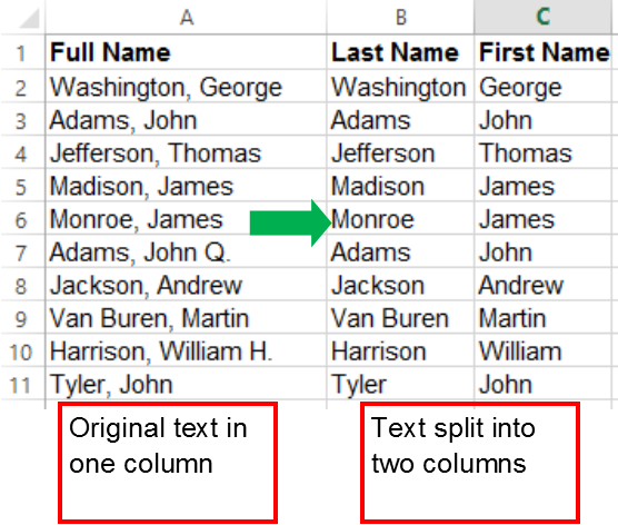
Cells within a worksheet that contain data, particularly textual data, can be merged or split as needed. While merging cells with textual data is a fairly common operation, splitting cells with data can prove more challenging as the split can impact the integrity of the data. The easiest way to split cells with textual data is to split columns rather than individually copying and pasting each piece of data to a new cell. This is particularly useful if you are working with a large data set that can be split into defined columns, such as splitting a single column of first and last names into two columns: one containing last names and the other containing first names.
To learn how to split cells with textual data, view the Split text into different cells article in the Microsoft Support Center.
Freeze panes in worksheet
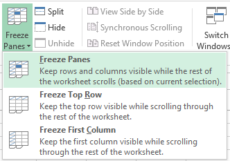
Worksheet display in Excel can be adjusted so that selected rows and columns can be frozen while the remaining rows and columns in the worksheet can be scrolled through. Freezing selected rows and columns in a worksheet is useful when it is necessary to keep select rows and columns in view while scrolling through data that has been entered in other rows or columns of the worksheet. The easiest way to freeze rows is to target a row or column that will remain visible. Then, select a cell below the targeted row or select a cell to the right of the targeted column and click the Freeze Panes icon in the View tab of the Ribbon. To freeze rows and columns, select a cell below the targeted row and adjacent to the targeted column before clicking the Freeze Panes icon.
To learn more about how to freeze panes, view the Freeze or lock rows and columns article in the Microsoft Support Center.
